Excel conditional formatting is an invaluable tool that allows the clear identification of various types of data. In fact, it saves a lot of time in making your raw data into information for easy decision making. If you are able to harness the power of conditional formatting, then chances are damn sure that you are making your entire work error free and very easier.
The awesome use of conditional formatting arises when you have a excel sheet filled with enormous amount of data with negative and positive figures. If your boss has given you a task to separate negative and positive figures, then you can use Excel conditional formatting very easy.
Excel conditional formatting red if negative green if positive Example
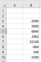
Consider an Excel worksheet that contains various figures, both positive and negative like below:

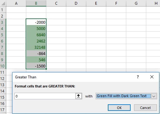
Now select the cells from B3 to B10. Now from Hone tab ribbon, click Conditional Formating > Highlight Cells Rules > Greater Than and put the value 0 in the field and choose Green Fill with Dark Green Text as shown in the image below:

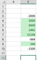
When you click Ok, you should see that positive figures have now converted into green cells as shown below in the image:

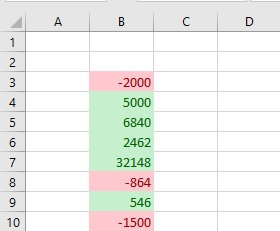
Now, select again the cells from B3 to B10 and click Conditional Formatting. This time, click Less Than from Highlight Cells Rules. Put the value 0 in the field and choose Light Red Fill with Dark Red Text. Upon doing so and cliking the OK button, you will have something like this. As you can see, figure/ values lower than 0 have now turned red. So, our mission is complete now.
Congratulations! we have learnt the art of formatting red if negative green if positive.
